Scientific expert classification

Introduction

SciLine is a non-profit organization hosted by the American Association for the Advancement of Science. SciLine’s mission is to get more credible scientific evidence into the news. The main service offered in the pursuit of this mission is expert matching, in which journalists reach out to SciLine to get connected with scientific experts to help them add evidence to their news stories. An example of these types of journalist requests is a reporter with the New York Times covering a local EPA groundwater contamination report asking for SciLine to connect them with a pollution expert. The experts which SciLine contacts are created as profiles in a database, allowing them to be found and used on future journalist requests received.

Expert profiles include descriptive text describing their expertise and are often labeled with one or more scientific disciplines, like “Pollution.” These disciplines allow SciLine to look at the overall distribution of scientific expertise within the database, and, among other uses, allows for the identification of major gaps in the database—highlighting disciplines which may need to be built out in terms of number of experts based on the disciplines each journalist request is labeled with. For example, SciLine gets many climatology-based requests for experts, but of the labeled experts in the database this discipline does not contain many experts.

One large problem SciLine faces is in the realm of data completeness. Many experts in the database lack any discipline labeling, meaning identification of gaps in the database (as well as useful information to find each expert for a given request) is not identifiable. Though manual work could be done to go through each expert profile and appropriately label each one with one or more disciplines, machine learning methods present a potentially more efficient strategy.

Analysis and Models

About the Dataset

The dataset comes directly from SciLine’s proprietary database and contains data from expert profiles. For the purposes of this project, personally identifiable information is removed, and only fields that contain relevant textual information are kept (including the discipline labels which will be used for the training and testing data)—along with the Contact ID to later go back and update discipline labels with predicted values.

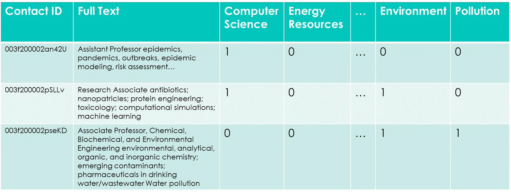
The dataset as a whole contains the approximately 11,500 experts which contain at least one discipline label. This encompasses 56% of the entire database size in terms of experts—further indicating the potential usefulness of this project. 44% of the experts in SciLine’s database contain no discipline label, highlighting a need to quickly classify these experts in order to better understand the distribution of experts SciLine has immediate access to. Three examples of expert profiles, and the data used for these models, is provided below:

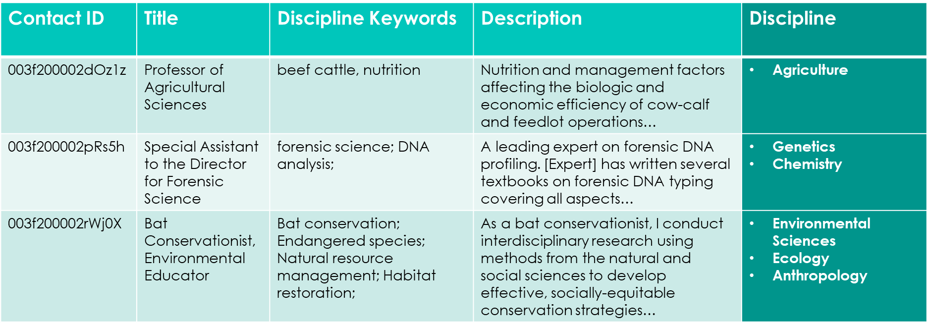
Since the information that is needed for use in the models is the textual data, Title, Discipline Keyword, and Description fields are concatenated into one field before further preprocessing. Disciplines and Contact IDs are kept separate for use in training and later use in taking the outputs of the models and tying them back to the individual expert profiles.

Overall, the purpose of using machine learning models on this data is three-fold: to predict the most accurate top-level discipline, to predict the most accurate secondary-level discipline, and to predict up to four secondary level disciplines per expert.

Document Size

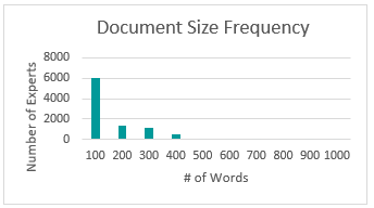
After concatenation, document size frequency was analyzed to determine the range of expert profile sizes in terms of word count. Using a subset of the data looking only at profiles containing one discipline label, it’s clear from a high level (right) that most expert profiles contain 100 or less words in their descriptive text. While thousands more contain 200-400 words, very few contain more than that many words.

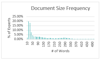
Looking at a smaller view, the distribution of expert profile size in words between 0 and 500 (left), and it’s apparent that over half of the experts reviewed contain fewer than 50 words of descriptive text, with most of the remainder falling between 50 and 300 words. The high number of profiles with fewer than 50 words indicates potential difficulties in correctly identifying discipline labels due to insufficient data.

About the Disciplines

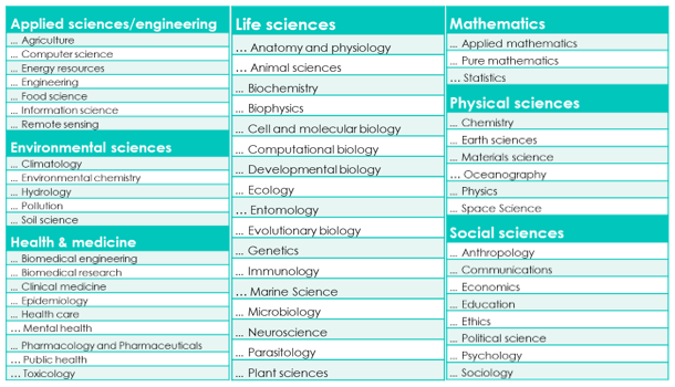
The discipline taxonomy used by SciLine in the labeling of experts includes seven top-level disciplines, and 55 secondary-level disciplines. Top level disciplines are useful in seeing broadly the distribution of experts in the database whereas secondary-level disciplines give more specific insight into potential gaps in the database, they also offer utility for SciLine staff in finding experts with specific expertise in the fulfillment of journalist requests. These can be seen below:

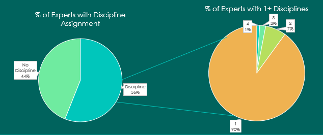
Experts can have up to four discipline labels, though very few have more than one. Over half (56%) of experts in the database contain a discipline label. Of the labeled experts, 90% of them only have one discipline label, with 7% containing 1 discipline labels, 2% containing three discipline labels, and just 1% containing four discipline labels. See chart below:

Similar to the distribution of word counts among the experts, the distribution of disciplines is also unbalanced. In looking at Top-Level disciplines (below) it’s clear that social science experts are disproportionally represented, with fewer than 5% of experts containing a mathematics or environmental science label.

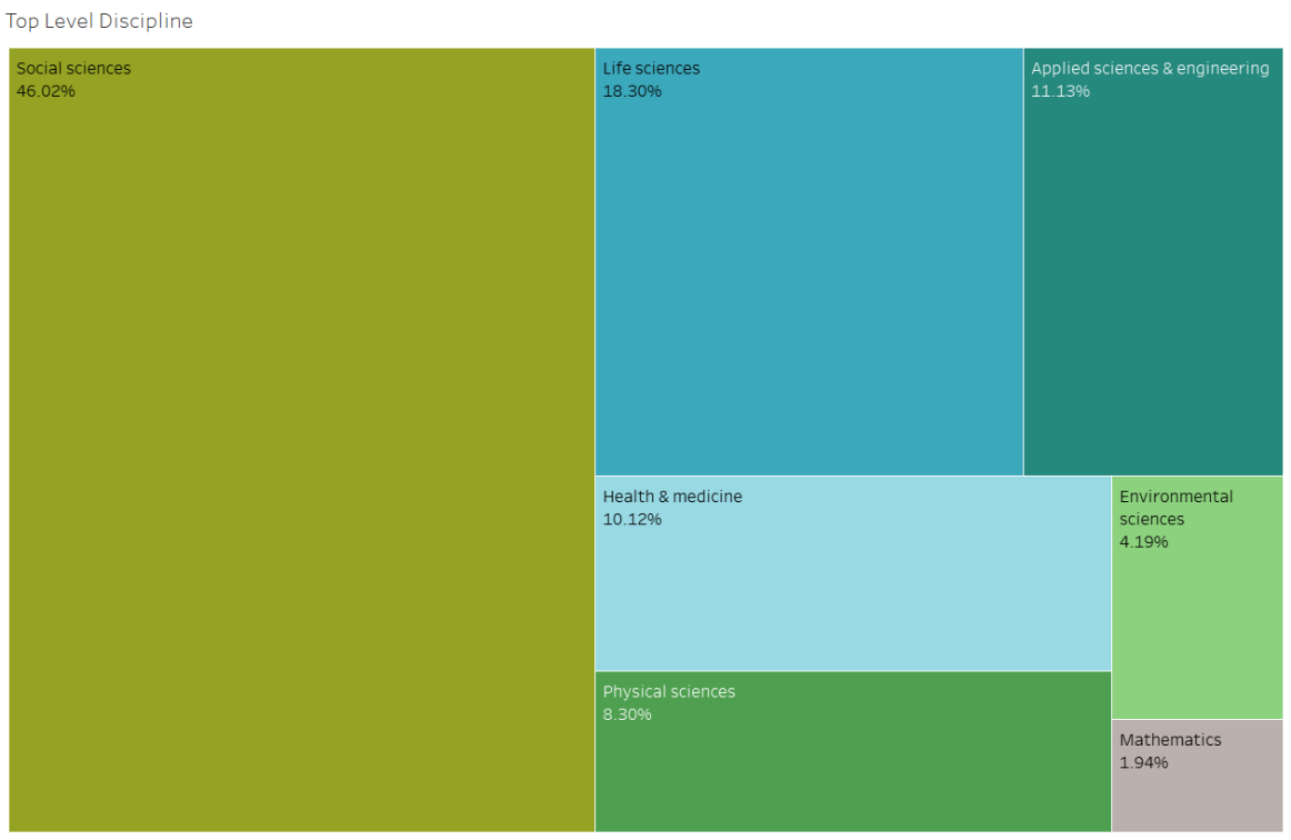
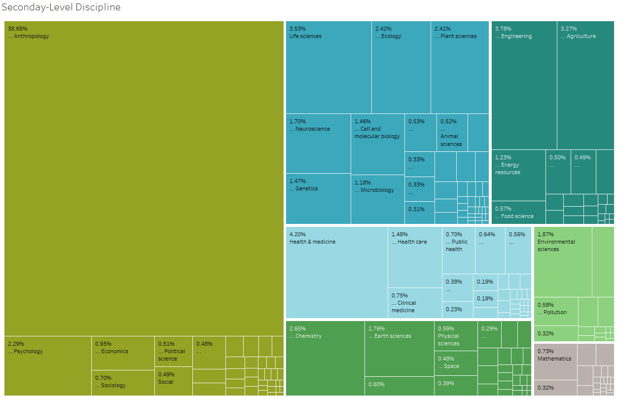
Looking at secondary-discipline distribution gives further insight into which disciplines are truly over (and under) represented in SciLine’s database. Anthropologists alone make up almost 40% of the database. It’s also apparent that in every top-level discipline category, there is wide variation in proportion of secondary-level disciplines.

Text Preprocessing:

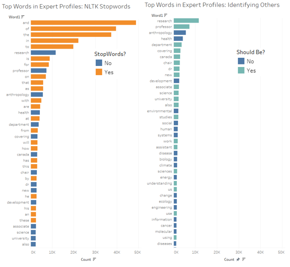
In order to reduce the dimensionality of the data processed by the model, the top words used across all expert profiles were derived to identify ones which do not impart information regarding discipline. In the first graph (below, left) it’s apparent that the majority of top words were those already identified as being commonly used by NLTK’s English stop word list (in orange.) Of the remaining words not previously identified by NLTK (below, right) highlighted in green are those which were determined to not be useful in discipline classification.

Words like research, professor, department, covering, chair, dr., science, university, and studies all are words used generically to describe scientists and where they word, as well as their title. These words, in addition to NLTK’s stop words, were then removed from all expert profiles.

Vectorization:

To find out which words are used most often, each expert’s descriptive text needs to be broken down into their constituent parts, the words themselves, and then counted. One way to do this is through one-hot encoding, or count vectorization.

Count vectorization takes all the words in all 10,000+ expert profiles and converts them to attributes each review can have a value for. For the descriptive text “A leading expert on forensic DNA profiling…” the attribute for “DNA” would have a value of 1. Because each expert text is often 100 words or fewer in length, and many words are used across all the experts, descriptive text will have a value of 0 for the vast majority of attributes. Though there are numerous ways to vectorize textual data, the CountVectorizer fulfills the function of counting the number of times a given word appears which is what is needed for the purpose of analyzing which terms are used most frequently.

Rather than using CountVectorizer, another option is using Term Frequency Inverse Document frequency (Tf-Idf), which, rather than counting the times a given word appears, weights each term by its prevalence in all the documents (expert descriptive texts.) This allows the model to more heavily weight infrequent words, and de-value common ones (like environment.)

A final vectorization method was used, taking count as well as bigrams, or two word pairs. For the above mentioned expert, “DNA profiling” would also be counted once, as would “forensic DNA.” This vectorization method expands the size of the data substantially, but helps get at more linguistic meaning in cases like “climate change” and “biological engineering.”

Data Sub-setting:

The purpose of using these models is three-fold: to predict the most accurate top-level discipline, to predict the most accurate secondary-level discipline, and to predict up to four secondary level disciplines per expert. These divergent purposes require different subsets and transformations of the data.

For the top-level classification, all experts with a single discipline label are taken, and in any case where that label is of the secondary-level, the overarching top-level is taken. For example, any expert labeled as “Public Health” would have that label transformed into “Health & medicine;” for any expert with the label “Materials Science,” that label would be transformed to be “Applied sciences & engineering.”

In order to compensate partially for the unbalanced nature of this dataset, experts labeled as “Social sciences” are then sampled down to be on par with the number of next largest discipline (Life Sciences.) This is to test if the models are too highly tuned to the largest category, or if they are actually easier to predict.

The third subset takes all experts with a single secondary-level discipline (ignoring any who experts who are only labeled, for example, “Health & medicine.”) This subset then removes a sample of the experts labeled as Anthropologists down to be on par with the size of the next largest label (Engineering.) A smaller sample, removing experts with disciplines that had less than 40 instances was also taken to address memory errors when using bigrams.

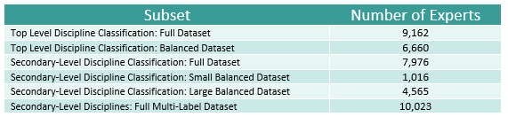
The sixth subset takes all experts with any secondary-level disciplines, removing all top-level disciplines, but considering all experts with multiple labels. This dataset is used in the One vs. Rest model for multi-label classification. A table below shows each subset and the number of experts within each record.

For multi-label classification using the OneVsRest classifier discussed below, further data transformation was needed. Rather than having a single attribute for “discipline,” all disciplines were converted to binary attributes, with each expert having up to four attributes containing a 1 with the rest containing 0s. This sparse matrix of data contained mainly 0s, given that the majority of experts had only one secondary discipline while there were 55 possible labels across the whole dataset. An example of the data after transformation can be seen below:

Testing and Training Data:

For all models, the common test-train split of 70%/30% is used, resulting in testing data sets as small as 305 experts, and as large as 3,000 experts. These training datasets were then used in different permutations of data subset, vectorization method, and n-gram length (testing unigrams and bigrams.)

Multi-Class Classification:

Naïve Bayes:

Naïve Bayes Classifiers are supervised machine learning models used to assign a class (in this case, scientific discipline) based on the probability of features (the words in the expert’s descriptive text) occurring in each class. For the classifier to work, the dataset is split into a training and testing set, with the training set’s labels being used to determine the prior probability of each word being in each category. Based on these prior probabilities, the model is used to predict what class each expert profile from the test data is in. The true test labels are then compared to determine how accurate the classifier was in its assignment.

For the top-level discipline classification, the unbalanced subsets were used with both CountVectorizer and Tf-Idf to determine best vectorization methods. Then the best vectorization method was used on the balanced dataset.

Support Vector Machine:

Linear Support Vector Classifiers are supervised machine learning models used to assign class (in this case, scientific discipline) based on an where an instance (in this case each expert’s descriptive text) lies in a vector space in relation to a hyperplane, which divides the data into categories. The hyperplane which divides the classes is determined by the training data, where the testing data falls in relation to this hyperplane of best fit then is used as the prediction. Using the same test-train split of 60%/40%, the SVM model was used first on the best vectorized data using the unbalanced then balanced dataset to determine overall accuracy.

Multi-Label Classification:

Multi-label classification is the task of labeling each instance (in this case, expert) with X labels from N possible classes, where X can be anywhere from 0 to N classes inclusive. In the case of this project, each expert can be labeled with up to 4 disciplines from 55 possible labels.

Naïve Bayes: One Vs. Rest:

The Naïve Bayes’ One Vs. Rest classifier takes the sparse matrix shown above and builds multiple classifiers for each expert instance, choosing all classes in which confidence is maximized. In the case of this project the task can be simplified to asking “is the expert an anthropologist?” then asking “is the expert an animal scientist?” without using the knowledge received in the first question to determine the answer to the second.

The main disadvantages to this type of model is that it assumes each secondary discipline is mutually exclusive. Since from institutional knowledge we know that a biomedical engineer is likely to also have expertise in another secondary-level discipline under the Health & medicine category, and an animal scientist is likely to not also be an anthropologist, this is an assumption that is not accurate, but one that may need to be accepted dependent on the accuracy of the results.

Naïve Bayes: Looking at Prior Probabilities:

A standard Naïve Bayes model can also be used in multi-label classification by looking at prior probabilities. Naïve Bayes takes the prior probability of each expert for each possible class, and predicts the label by selecting the highest probability. By printing each prior probability, the top 4 probabilities can be selected to label the expert with more than one discipline. An important addendum to this task if finding an appropriate threshold—at what prior probability should additional disciplines be selected? While this problem demands further input from SciLine stakeholders, it can also be ignored for the purposes of recommending discipline labels. That way a manual step in the process can be added in real time to suggest discipline labels for each expert after input.

Results:

Metrics of Success:

Accuracy is an important metric to determine overall quality and determining among models which is the strongest, but beyond model comparison precision is a more important metric. Precision indicates among all predictions in one category, how many are correct. While recall measures the ability of the model to find all the relevant cases within the test dataset, for the purposes of efficiently building out SciLine’s database, it’s more important to accurately assign labels (precision) that to classify many experts (recall). For this reason even if a model results in low recall for a given discipline, if the model shows high confidence in the experts it does classify, that is still readily useable information for building out the database.

Multi-Class Classification

Top-Level Discipline: Unbalanced Subset

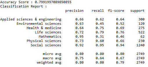
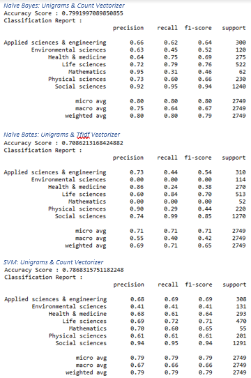
In using the top-level discipline subset on the full dataset (unbalanced), the count vectorizer model using unigrams resulted in the highest accuracy—79.9%. Given that the Tf-Idf vectorization model on the same dataset resulted in a significantly lower accuracy (70.8%), the count vectorizer was used for all other models. Using a Linear Support Vector Classifier resulted in a slightly lower accuracy of 78.6%. The Count Vectorized Naïve Bayes model also had the highest precision average—the metric that has the strongest bearing on utility for SciLine. See the table (below) for accuracy and weighted average precision scores. For the full classification report for each model see Appendix A.

Top-Level Discipline: Balanced Subset

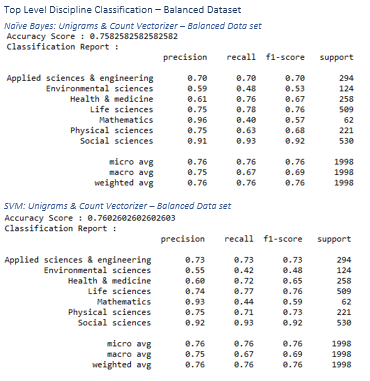
In using the top-level discipline subset that has removed a large portion of social scientists, somewhat balancing the dataset, the Linear SVM model resulted in a marginally higher accuracy of 76% in comparison to the Naïve Bayes model, which had an accuracy of 75.8%. Both models, however resulted in a 76% average precision score.

An important note on these models in comparison to the unbalanced models above is that the precision and recall scores for Social sciences classification were only marginally lower (95% in the unbalanced dataset, and 93% in the balanced dataset.) This indicates one of two possibilities: this subset is still too unbalanced and overly tuned to social sciences, or that social sciences are truly easier to predict.

Because a fully stratified sampling of the full dataset (taking just 178 rows per top-level discipline, given that that is how many experts are contained with the lowest populated discipline, mathematics) would result in a just 1,246 rows, not even 20% of the full dataset, this method was avoided. Thus the unbalanced models are preferred given that their results do not strongly differ from the balanced models outside of a slightly lower accuracy score. See the table (below) for accuracy and weighted average precision scores. For the full classification report for each model see Appendix B.

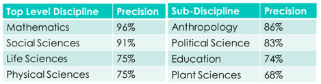
Overall, for top-level discipline classification, Naïve Bayes using the unbalanced dataset, count vectorizer, and unigrams resulted in the best results. From the classification report of this model (below) it is clear that, using the metric of precision, Mathematics, Social Sciences, Life sciences, and Physical sciences have the highest scores (over 70%.) Though the threshold for use needs to be determined by SciLine staff before use in building out the expert profiles, these disciplines are the best candidates for use.

Second Level Discipline Classification: Unbalanced Subset

The secondary-level discipline classification resulted in lower accuracies, which makes sense given that the data subset was smaller than in the top-level discipline classification, and that there were almost eight times more label possibilities.

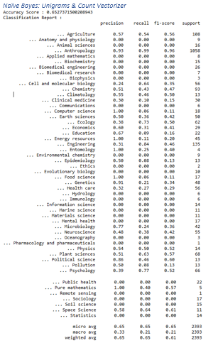
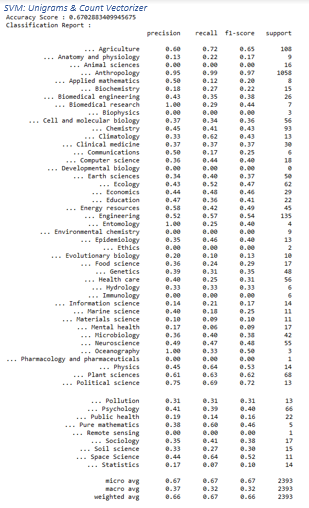
Using the unbalanced data set resulted in many less-populated disciplines to score a 0 in precision and recall, because the support for these classes was too low (under 10 in the test data). That being said for the higher populated classes, like Anthropology, Engineering, political science, and neuroscience, precision scores varied between 45% and 100% (energy resources.) Using the unbalanced data set, the Linear SVC perfomed marginally better, with an accuracy of 67% (compared to 65.3% in Naïve Bayes) and 66% precision score (compared to 65%) The support for the largest discipline class (Anthropology) was almost ten times larger than the next most popular class (engineering)—further highlighting the need to test a more balanced data set. See the table (below) for accuracy and precision scores for these models, and Appendix C for the classification reports.

Second Level Discipline Classification: Small Balanced Subset

In order to test bigrams, which significantly increase the dimensionality of the dataset by taking both single terms and two-word pairs, the second level discipline data was further subset by reducing the number of anthropologists down to be on par with the next largest sample (engineering) and then removing all experts with a discipline which totaled less than 40 instances, or experts.

Because this dataset was approximately 1/7th the full unbalanced dataset, accuracy scores were lower, but some interesting results did arise.

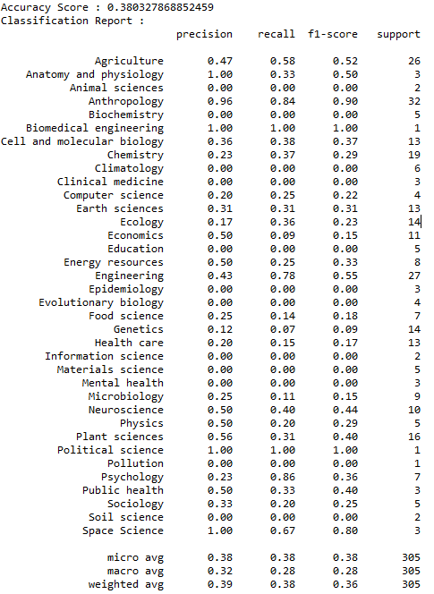
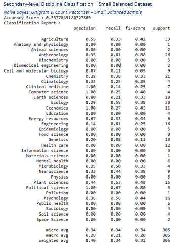
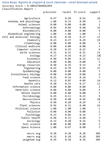
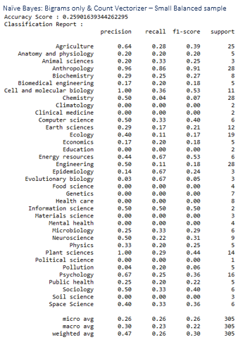
Testing the Naïve Bayes model using the count vectorizer on unigrams resulted in an accuracy of 33.8%, incorporating bigrams resulted in a higher accuracy score of 38%, though using bigrams alone resulted in the lowest accuracy score of 25.9%. The bigram and unigram model did not result in the highest precision score, which was 40% in the unigram model. See the table below for accuracy and precision scores in the small balanced data set, and Appendix D for the classification reports.

The use of bigrams increased precision across numerous secondary disciplines, including Anatomy and Physiology, which went from 0% to 100%. Anthropology is consistently well predicted, as is biomedical engineering, political science, and space science. See below for the classification report of this model. In all of those secondary disciplines the precision score was above 90%. Among these models the use of unigrams and bigrams proved most successful, influencing the use of this vectorization method for the next set of models—the large balanced subset.

Second Level Discipline Classification: Large Balanced Subset

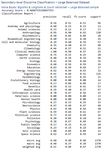
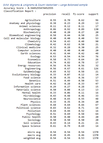
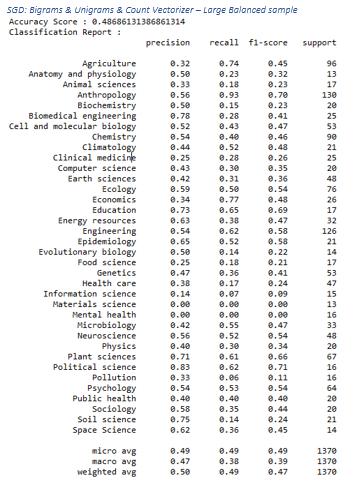
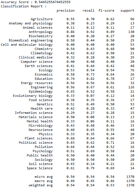
Expanding the initial balanced dataset by incorporating more expert profiles (increasing the dataset from 1,016 to 4,565) and maintaining bigrams and unigrams, Naïve Bayes was compared to Linear SVC, and to an SVM model using Stochastic Gradient Descent. The Linear SVC resulted in the highest accuracy, 54.4% in comparison to Naïve Bayes’ 48.5% and SGD’s 48.6% See table below for precision and accuracy scores using this subset. See Appendix E for classification reports.

Though the accuracy did not reach as high as the levels seen in the models using the full unbalanced dataset, Anthropology still saw very high precision and recall (86% and 92% respectively.) Certain secondary-level disciplines, including political science and education, stuck out as having higher than 70% precision scores—highlighting that social sciences generally are easier to classify. From the classification report for the highest scoring model using this model (Linear SVC) see below:

Multi-Class Classification: Major Takeaways

Overall, it is clear that the larger, unbalanced dataset again resulted in the highest accuracy scores—and from the consistently high scores Anthropology received in precision and recall across all subsets, it appears that the models were not overly tuning for this category—but that social sciences generally were the most accurate to predict. Further evidence for this result can be seen through looking into the top words in the social science categories which had the strongest results:

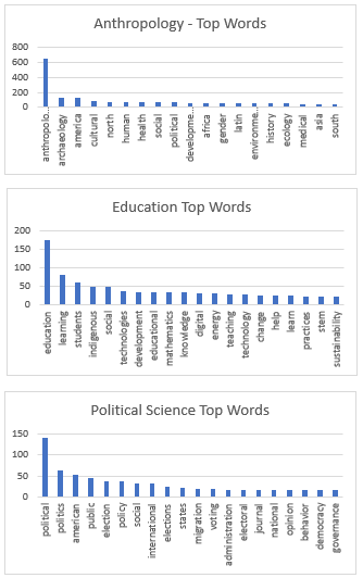
In looking at the top words for anthropology (after removing previously identified stop words), most of the top terms are ones that fit firmly within anthropology, and anthropology alone.

Archeaology, America, cultural, social, gender, and history are all terms that are not vague in their association with discipline—giving evidence to why the models were good at classifying this secondary discipline.

In looking at the top words for education, the same scenario unfolds. Education, learning, students, educational, knowledge, teaching and learn are all terms which fit squarely within the education discipline, with few terms, like mathematics, appearing which could just as easily be associated with another discipline.

Political science shows a third example: political, politics, public, election, policy, international, elections, voting and electoral are all terms closely associated with the field of political science, with only social spanning multiple discipline areas.

In looking at other secondary-level disciplines which were not well-predicted by the models, the opposite can be seen. In animal sciences, the top words include terms like ecology, brain, development, environmental, quantum, and health (in orange) which are all more closely associated with disciplines like ecology, neuroscience, physics, and public health. Material sciences shows a similar scenario, with energy, engineering, cells, molecules, and molecular appearing which could just as easily appear under other disciplines, like energy resources, cell and molecular biology, or engineering.

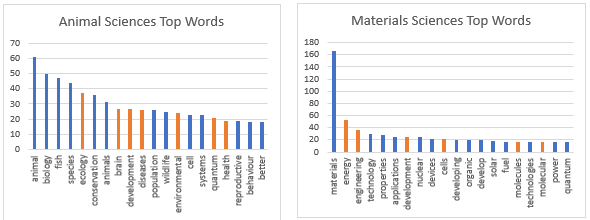
These top-word analyses also provide insight into why the bigram models resulted in a higher accuracy—biomedical engineering is a discipline of its own while “biomedicine” or “engineering” could relate to entirely separate categories. This shows that the use of bigrams in addition to unigrams is worth the added dimensionality to further the model’s understanding of the expert’s description.

With more memory capacity, it would be useful to run a final model, using 100% of the data as the training data set to determine which top-level and secondary-level disciplines are best predicted for, then using the precision scores for each possible class to determine which predictions meet the threshold set by SciLine staff for use in building out the database. From the initial results from all models using testing data, the following top and secondary-level disciplines should be the preferred ones for use in classifying unlabeled expert profiles:

Multi-Label Classification:

Naïve Bayes One vs rest:

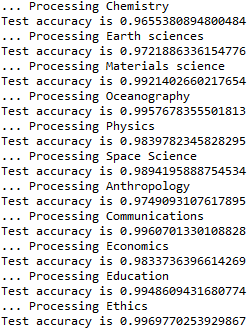
In using the full multi-labeled subset of data, transformed to have binary attributes for each possible secondary-level discipline, the accuracy for classifying each expert as either a “1” or “0” for each class resulted in incredible high accuracy: up to 100% in some cases but for all labels the accuracy was in the high 90s (see a snapshot of the accuracy scores for some of these disciplines in the report to the right.)

However, these accuracies are not a good measure of how well the model is performing. Because the data set is a sparsely populated matrix, with the majority of label values being 0 for each expert and only a few (mostly one) label having a value of 1, the model tends to assume that all labels are 0 for all experts. This is further highlighted by anthropologies slightly lower accuracy (97%.) This is because the model is assuming very few experts are anthropology, which is correct, but it assumes too few have that label—resulting in the proportionally lower accuracy in comparison to Ethics, for example, which had a 99.7% score.

Overall, the One vs. Rest model did not result in actionable predictions for use at SciLine, but lead to the need to adapt the previously tested standard Naïve Bayes models for use in assigning multiple classes, or disciplines.

Pseudo-multi-label classification: Conditional Probabilities

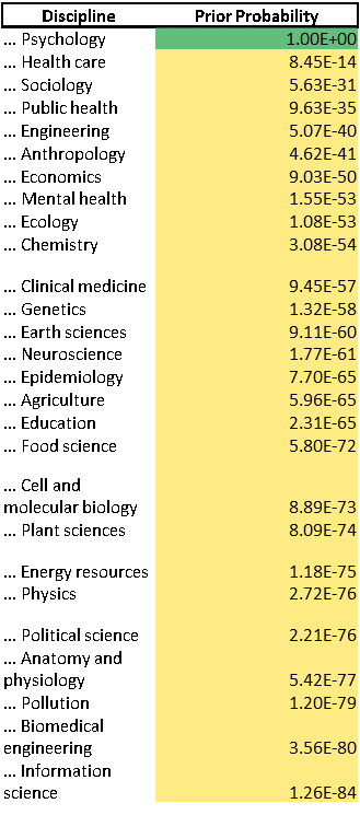
Given that Naïve Bayes takes the conditional probability of each expert for each possible class, and predicts the label by selecting the highest probability, by printing each probability, the top 4 probabilities can be selected to label the expert with more than one discipline. Testing this method on the first expert gives the results shown to the right.

While this expert was predicted to be a psychologist, health care, sociology, and public health also scored relatively high in regard to their prior probability. In looking at the expert’s descriptive text (below) these other top probable disciplines appear to, at some degree, apply:

Director of Psycho-Oncology, Clinical Psychologist. As I Clinical Psychologist, I specialize in treating anxiety, depression, and helping patients cope with cancer.My current research is focused on developing and testing a mhealth mobile application for caregivers and patients with advanced cancer. Psycho-Oncology, Caregiver Stress, Sexual Dysfunction, Anxiety, Depression, Technological Intervention Development and Dissemination (mhealth), Cognitive Behavioral Therapy, Exposure Therapy, Coping with Cancer, women's sexual health, adolescent anxiety.

While sociology may not be a perfect fit, health care and public health are clearly relevant labels to this expert given their descriptive text. This method of using Naïve Bayes’ produced prior-probabilities shows immediate use in application at SciLine. By taking all labeled data and finding the top-n scoring labels for each, recommendations can be made to a manual reviewer for label assignment. With further input from SciLine staff on setting a threshold for prior probabilities, manual work could be removed entirely and any labels meeting the threshold could be then used to automatically populate labeled and unlabeled data.

The main drawback to this method, however, is that it relies on single-labeled datasets. This means that as SciLine continues to build out the database with multiple labels, only one label for each expert could be used in the training of the model.

Multi-Label Classification: Major Takeaways

The next steps needed for implementation would be to run a final model on all labeled data, using bigrams which would demand a higher memory capacity, and then use that model to predict label conditional probabilities for all unlabeled and labeled data. From there, using a pre-determined probability threshold would give immediate results, printing all top-scoring labels for each expert. This data could then be used immediately for updating the database, or reviewed in batches to ensure more accurate input before bulk uploading the updated data to the database for use.

Discipline classification of scientific experts is not a straightforward process, and there remains a large variability among the disciplines themselves regarding which can accurately be predicted using machine learning. While the social sciences appear to be the most easily classified, many natural and applied sciences, including the biosciences and engineering, often overlap in regard to the words used to describe that type of expertise. That being said, low levels of success depending on the discipline predicted does not mean failure across the board. Based on the precision scores of each discipline, high-scoring labels can still be considered in the task of building out profiles. If the models do not predict animal scientists well then that’s fine, those predictions will not be used to build out the database. But for many social science disciplines, which are very precise regarding their predictions, the results of these models can serve an immediate function in their use at SciLine.

Conclusion:

SciLine relies on an expansive database of scientific experts to function in the service of getting more scientific evidence in the news. Which disciplines each expert is associated with is an important piece of information for SciLine—both in the ability for SciLine staff to quickly find an expert for a journalist’s request, and in more descriptive task of identifying disciplines that need to have more experts added to compensate with large numbers of requests in that field.

While the manual assignment of disciplines by qualified and experienced staff remains the best way to generate this information, machine learning offers another method to fill in gaps in key areas. Where these methods currently excel is in their ability to assign experts to labels in the social sciences—an important area for SciLine given the amount of requests journalists send in asking about sociological and political questions. Because one of the largest problems SciLine faces is in the realm of data completeness, any opportunity to efficiently label experts in any field is a boon for productivity—highlighting the fact that even if machine learning does not present the perfect solution, any solution can help.

Having discipline-labeled experts in the database also allows SciLine to tell interesting, and timely, stories. With coronavirus and the disease it causes, COVID-19, currently taking up the vast majority of air time on TV and text space in newspapers, SciLine has experienced a surge in requests for experts in epidemiology, public health, and related fields. Having labeled experts gives SciLine the opportunity to look back and be able to see, from a top level, how the national conversation has changed as the pandemic has gone on over time. An example, which uses estimates rather than true figures, is shown below:

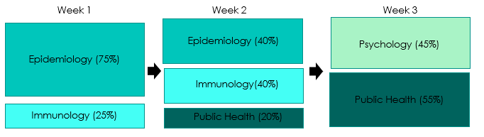
In the beginning of the outbreak in the United States, journalists wanted to hear from epidemiologists and immunologists to talk to them about the virus itself—how it propagates, it’s origins, and similar cases like SARS and MERS in the past. But as time went on, and the disease started to impact more people on a more human level, journalists started to want to hear from public health experts—asking questions about how the public health system can respond, overall load on the system, and emerging conversations about “flattening the curve.” More recently however, journalists have begun to ask for help finding psychologists and social scientists to discuss how COVID-19 is impacting social life, what the mental health impacts of social isolation are, and what individuals can do to keep themselves and their loved ones safe.

This type of storytelling relies on SciLine tracking the scientific disciplines of the experts whom they refer to journalists every day. While ensuring that staff continually update and maintain expert profiles as they’re used to fulfill journalist requests will always be important, machine learning models offer an additional method to quickly and precisely back-fill incomplete data.